四阶龙格库塔法 - 扩散方程 - 图像分析
4th Order Runga Kutta Method - Diffusion equation - Image analysis
这是速度的问题。我正在尝试求解具有三个行为状态的扩散方程,其中:
- Lambda == 0 平衡
- Lambda > 0 最大扩散
- Lambda < 0 分钟扩散
瓶颈是扩散运算符函数中的else语句
平衡态有一个简单的T算子和扩散算子。对于其他两个州来说,它变得相当复杂。到目前为止,我还没有耐心看完代码 运行 次。据我所知方程是正确的,平衡状态的输出看起来是正确的,也许有人有一些技巧可以提高非平衡状态的速度?
(我想用欧拉解 (FTCS) 代替 Runge-Kutta 会更快。还没试过。)
您可以导入任何黑白图像来试用代码。
import numpy as np
import sympy as sp
import scipy.ndimage.filters as flt
from PIL import Image

# import image
im = Image.open("/home/will/Downloads/zebra.png")
arr = np.array(im)
arr=arr/253.

def T(lamda,x):
    """
    T Operator
    lambda is a "steering" constant between 3 behavior states
    -----------------------------
    0     -> linearity
    +inf  -> max
    -inf  -> min
    -----------------------------
    """
    if lamda == 0:  # linearity
        return x
    elif lamda > 0: #  Half-wave rectification
        return np.max(x,0)
    elif lamda < 0: # Inverse half-wave rectification
        return np.min(x,0)


def Diffusion_operator(lamda,f,t):
    """
    2D Spatially Discrete Non-Linear Diffusion
    ------------------------------------------
    Special case where lambda == 0, operator becomes Laplacian


    Parameters
    ----------
    D : int                      diffusion coefficient
    h : int                      step size
    t0 : int                     stimulus injection point
    stimulus : array-like        luminance distribution

    Returns
    ----------
    f : array-like               output of diffusion equation
    -----------------------------
    0     -> linearity (T[0])
    +inf  -> positive K(lamda)
    -inf  -> negative K(lamda)
    -----------------------------
    """
    if lamda == 0:  # linearity
        return flt.laplace(f)
    else:           # non-linearity
        f_new = np.zeros(f.shape)
        for x in np.arange(0,f.shape[0]-1):
            for y in np.arange(0,f.shape[1]-1):
                f_new[x,y]=T(lamda,f[x+1,y]-f[x,y]) + T(lamda,f[x-1,y]-f[x,y]) + T(lamda,f[x,y+1]-f[x,y])
                + T(lamda,f[x,y-1]-f[x,y])
        return f_new


def Dirac_delta_test(tester):
    # Limit injection to unitary multiplication, not infinite
    if np.sum(sp.DiracDelta(tester)) == 0:
        return 0
    else:
        return 1

def Runge_Kutta(stimulus,lamda,t0,h,N,D,t_N):
    """
    4th order Runge-Kutta solution to:
    linear and spatially discrete diffusion equation (ignoring leakage currents)

    Adiabatic boundary conditions prevent flux exchange over domain boundaries
    Parameters
    ---------------
    stimulus : array_like   input stimuli [t,x,y]
    lamda : int             0 +/- inf
    t0 : int                point of stimulus "injection"
    h : int                 step size
    N : int                 array size (stimulus.shape[1])
    D : int                 diffusion coefficient [constant]

    Returns
    ----------------
    f : array_like          computed diffused array

    """
    f = np.zeros((t_N+1,N,N)) #[time, equal shape space dimension]
    t = np.zeros(t_N+1)

    if lamda ==0:
        """    Linearity    """
        for n in np.arange(0,t_N):
            k1 = D*flt.laplace(f[t[n],:,:]) +     stimulus*Dirac_delta_test(t[n]-t0)
            k1 = k1.astype(np.float64)
            k2 = D*flt.laplace(f[t[n],:,:]+(0.5*h*k1)) +     stimulus*Dirac_delta_test((t[n]+(0.5*h))- t0)
            k2 = k2.astype(np.float64)
            k3 = D*flt.laplace(f[t[n],:,:]+(0.5*h*k2)) + stimulus*Dirac_delta_test((t[n]+(0.5*h))-t0)
            k3 = k3.astype(np.float64)
            k4 = D*flt.laplace(f[t[n],:,:]+(h*k3)) + stimulus*Dirac_delta_test((t[n]+h)-t0)
            k4 = k4.astype(np.float64)
            f[n+1,:,:] = f[n,:,:] + (h/6.) * (k1 + 2.*k2 + 2.*k3 + k4)
            t[n+1] = t[n] + h
        return f

    else:
        """    Non-Linearity   THIS IS SLOW  """
        for n in np.arange(0,t_N):
            k1 = D*Diffusion_operator(lamda,f[t[n],:,:],t[n]) + stimulus*Dirac_delta_test(t[n]-t0)
            k1 = k1.astype(np.float64)
            k2 = D*Diffusion_operator(lamda,(f[t[n],:,:]+(0.5*h*k1)),t[n]) + stimulus*Dirac_delta_test((t[n]+(0.5*h))- t0)
            k2 = k2.astype(np.float64)
            k3 = D*Diffusion_operator(lamda,(f[t[n],:,:]+(0.5*h*k2)),t[n]) + stimulus*Dirac_delta_test((t[n]+(0.5*h))-t0)
            k3 = k3.astype(np.float64)
            k4 = D*Diffusion_operator(lamda,(f[t[n],:,:]+(h*k3)),t[n]) + stimulus*Dirac_delta_test((t[n]+h)-t0)
            k4 = k4.astype(np.float64)
            f[n+1,:,:] = f[n,:,:] + (h/6.) * (k1 + 2.*k2 + 2.*k3 + k4)
            t[n+1] = t[n] + h

        return f

# Code to run
N=arr.shape[1]  # Image size
stimulus=arr[0:N,0:N,1]
D = 0.3   # Diffusion coefficient [0>D>1]
h = 1     # Runge-Kutta step size [h > 0]
t0 = 0    # Injection time
t_N = 100 # End time

f_out_equil = Runge_Kutta(stimulus,0,t0,h,N,D,t_N)
f_out_min = Runge_Kutta(stimulus,-1,t0,h,N,D,t_N)
f_out_max = Runge_Kutta(stimulus,1,t0,h,N,D,t_N)
简而言之,f_out_equil 的计算速度相对较快,而 min 和 max 的情况既昂贵又缓慢。
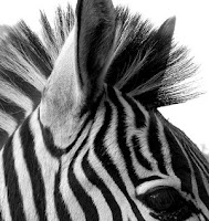
这是我一直在使用的图像的 link:http://4.bp.blogspot.com/_KbtOtXslVZE/SweZiZWllzI/AAAAAAAAAIg/i9wc-yfdW78/s200/Zebra_Black_and_White_by_Jenvanw.jpg
感谢有关改进编码的提示,
非常感谢,
这是输出的快速绘图脚本
import matplotlib.pyplot as plt
fig1, (ax1,ax2,ax3,ax4,ax5) = plt.subplots(ncols=5, figsize=(15,5))
ax1.imshow(f_out_equil[1,:,:],cmap='gray')
ax2.imshow(f_out_equil[t_N/10,:,:],cmap='gray')
ax3.imshow(f_out_equil[t_N/2,:,:],cmap='gray')
ax4.imshow(f_out_equil[t_N/1.5,:,:],cmap='gray')
ax5.imshow(f_out_equil[t_N,:,:],cmap='gray')
python 中的 For 循环往往很慢;您可以通过尽可能多地矢量化来获得巨大的加速。 (这将对你解决未来的任何数字问题有很大帮助)。新的 T 运算符同时处理整个数组,并且在 Diffusion_operator 中调用 np.roll 将图像数组正确排列以进行有限差分计算。
整个过程 运行 在我的电脑上大约 10 秒。
def T(lamda,x):
    """
    T Operator
    lambda is a "steering" constant between 3 behavior states
    -----------------------------
    0     -> linearity
    +inf  -> max
    -inf  -> min
    -----------------------------
    """
    if lamda == 0:  # linearity
        return x
    elif lamda > 0: #  Half-wave rectification
        maxval = np.zeros_like(x)
        return np.array([x, maxval]).max(axis=0)
    elif lamda < 0: # Inverse half-wave rectification
        minval = np.zeros_like(x)
        return np.array([x, minval]).min(axis=0)


def Diffusion_operator(lamda,f,t):
    """
    2D Spatially Discrete Non-Linear Diffusion
    ------------------------------------------
    Special case where lambda == 0, operator becomes Laplacian


    Parameters
    ----------
    D : int                      diffusion coefficient
    h : int                      step size
    t0 : int                     stimulus injection point
    stimulus : array-like        luminance distribution

    Returns
    ----------
    f : array-like               output of diffusion equation
    -----------------------------
    0     -> linearity (T[0])
    +inf  -> positive K(lamda)
    -inf  -> negative K(lamda)
    -----------------------------
    """
    if lamda == 0:  # linearity
        return flt.laplace(f)
    else:           # non-linearity
        f_new = T(lamda,np.roll(f,1, axis=0) - f) \
                + T(lamda,np.roll(f,-1, axis=0) - f) \
                + T(lamda,np.roll(f, 1, axis=1) - f) \
                + T(lamda,np.roll(f,-1, axis=1) - f)
        return f_new
这是速度的问题。我正在尝试求解具有三个行为状态的扩散方程,其中:
- Lambda == 0 平衡
- Lambda > 0 最大扩散
- Lambda < 0 分钟扩散
瓶颈是扩散运算符函数中的else语句
平衡态有一个简单的T算子和扩散算子。对于其他两个州来说,它变得相当复杂。到目前为止,我还没有耐心看完代码 运行 次。据我所知方程是正确的,平衡状态的输出看起来是正确的,也许有人有一些技巧可以提高非平衡状态的速度?
(我想用欧拉解 (FTCS) 代替 Runge-Kutta 会更快。还没试过。)
您可以导入任何黑白图像来试用代码。
import numpy as np
import sympy as sp
import scipy.ndimage.filters as flt
from PIL import Image
# import image
im = Image.open("/home/will/Downloads/zebra.png")
arr = np.array(im)
arr=arr/253.
def T(lamda,x):
"""
T Operator
lambda is a "steering" constant between 3 behavior states
-----------------------------
0 -> linearity
+inf -> max
-inf -> min
-----------------------------
"""
if lamda == 0: # linearity
return x
elif lamda > 0: # Half-wave rectification
return np.max(x,0)
elif lamda < 0: # Inverse half-wave rectification
return np.min(x,0)
def Diffusion_operator(lamda,f,t):
"""
2D Spatially Discrete Non-Linear Diffusion
------------------------------------------
Special case where lambda == 0, operator becomes Laplacian
Parameters
----------
D : int diffusion coefficient
h : int step size
t0 : int stimulus injection point
stimulus : array-like luminance distribution
Returns
----------
f : array-like output of diffusion equation
-----------------------------
0 -> linearity (T[0])
+inf -> positive K(lamda)
-inf -> negative K(lamda)
-----------------------------
"""
if lamda == 0: # linearity
return flt.laplace(f)
else: # non-linearity
f_new = np.zeros(f.shape)
for x in np.arange(0,f.shape[0]-1):
for y in np.arange(0,f.shape[1]-1):
f_new[x,y]=T(lamda,f[x+1,y]-f[x,y]) + T(lamda,f[x-1,y]-f[x,y]) + T(lamda,f[x,y+1]-f[x,y])
+ T(lamda,f[x,y-1]-f[x,y])
return f_new
def Dirac_delta_test(tester):
# Limit injection to unitary multiplication, not infinite
if np.sum(sp.DiracDelta(tester)) == 0:
return 0
else:
return 1
def Runge_Kutta(stimulus,lamda,t0,h,N,D,t_N):
"""
4th order Runge-Kutta solution to:
linear and spatially discrete diffusion equation (ignoring leakage currents)
Adiabatic boundary conditions prevent flux exchange over domain boundaries
Parameters
---------------
stimulus : array_like input stimuli [t,x,y]
lamda : int 0 +/- inf
t0 : int point of stimulus "injection"
h : int step size
N : int array size (stimulus.shape[1])
D : int diffusion coefficient [constant]
Returns
----------------
f : array_like computed diffused array
"""
f = np.zeros((t_N+1,N,N)) #[time, equal shape space dimension]
t = np.zeros(t_N+1)
if lamda ==0:
""" Linearity """
for n in np.arange(0,t_N):
k1 = D*flt.laplace(f[t[n],:,:]) + stimulus*Dirac_delta_test(t[n]-t0)
k1 = k1.astype(np.float64)
k2 = D*flt.laplace(f[t[n],:,:]+(0.5*h*k1)) + stimulus*Dirac_delta_test((t[n]+(0.5*h))- t0)
k2 = k2.astype(np.float64)
k3 = D*flt.laplace(f[t[n],:,:]+(0.5*h*k2)) + stimulus*Dirac_delta_test((t[n]+(0.5*h))-t0)
k3 = k3.astype(np.float64)
k4 = D*flt.laplace(f[t[n],:,:]+(h*k3)) + stimulus*Dirac_delta_test((t[n]+h)-t0)
k4 = k4.astype(np.float64)
f[n+1,:,:] = f[n,:,:] + (h/6.) * (k1 + 2.*k2 + 2.*k3 + k4)
t[n+1] = t[n] + h
return f
else:
""" Non-Linearity THIS IS SLOW """
for n in np.arange(0,t_N):
k1 = D*Diffusion_operator(lamda,f[t[n],:,:],t[n]) + stimulus*Dirac_delta_test(t[n]-t0)
k1 = k1.astype(np.float64)
k2 = D*Diffusion_operator(lamda,(f[t[n],:,:]+(0.5*h*k1)),t[n]) + stimulus*Dirac_delta_test((t[n]+(0.5*h))- t0)
k2 = k2.astype(np.float64)
k3 = D*Diffusion_operator(lamda,(f[t[n],:,:]+(0.5*h*k2)),t[n]) + stimulus*Dirac_delta_test((t[n]+(0.5*h))-t0)
k3 = k3.astype(np.float64)
k4 = D*Diffusion_operator(lamda,(f[t[n],:,:]+(h*k3)),t[n]) + stimulus*Dirac_delta_test((t[n]+h)-t0)
k4 = k4.astype(np.float64)
f[n+1,:,:] = f[n,:,:] + (h/6.) * (k1 + 2.*k2 + 2.*k3 + k4)
t[n+1] = t[n] + h
return f
# Code to run
N=arr.shape[1] # Image size
stimulus=arr[0:N,0:N,1]
D = 0.3 # Diffusion coefficient [0>D>1]
h = 1 # Runge-Kutta step size [h > 0]
t0 = 0 # Injection time
t_N = 100 # End time
f_out_equil = Runge_Kutta(stimulus,0,t0,h,N,D,t_N)
f_out_min = Runge_Kutta(stimulus,-1,t0,h,N,D,t_N)
f_out_max = Runge_Kutta(stimulus,1,t0,h,N,D,t_N)
简而言之,f_out_equil 的计算速度相对较快,而 min 和 max 的情况既昂贵又缓慢。
这是我一直在使用的图像的 link:http://4.bp.blogspot.com/_KbtOtXslVZE/SweZiZWllzI/AAAAAAAAAIg/i9wc-yfdW78/s200/Zebra_Black_and_White_by_Jenvanw.jpg
感谢有关改进编码的提示, 非常感谢,
这是输出的快速绘图脚本
import matplotlib.pyplot as plt
fig1, (ax1,ax2,ax3,ax4,ax5) = plt.subplots(ncols=5, figsize=(15,5))
ax1.imshow(f_out_equil[1,:,:],cmap='gray')
ax2.imshow(f_out_equil[t_N/10,:,:],cmap='gray')
ax3.imshow(f_out_equil[t_N/2,:,:],cmap='gray')
ax4.imshow(f_out_equil[t_N/1.5,:,:],cmap='gray')
ax5.imshow(f_out_equil[t_N,:,:],cmap='gray')
python 中的 For 循环往往很慢;您可以通过尽可能多地矢量化来获得巨大的加速。 (这将对你解决未来的任何数字问题有很大帮助)。新的 T 运算符同时处理整个数组,并且在 Diffusion_operator 中调用 np.roll 将图像数组正确排列以进行有限差分计算。
整个过程 运行 在我的电脑上大约 10 秒。
def T(lamda,x):
"""
T Operator
lambda is a "steering" constant between 3 behavior states
-----------------------------
0 -> linearity
+inf -> max
-inf -> min
-----------------------------
"""
if lamda == 0: # linearity
return x
elif lamda > 0: # Half-wave rectification
maxval = np.zeros_like(x)
return np.array([x, maxval]).max(axis=0)
elif lamda < 0: # Inverse half-wave rectification
minval = np.zeros_like(x)
return np.array([x, minval]).min(axis=0)
def Diffusion_operator(lamda,f,t):
"""
2D Spatially Discrete Non-Linear Diffusion
------------------------------------------
Special case where lambda == 0, operator becomes Laplacian
Parameters
----------
D : int diffusion coefficient
h : int step size
t0 : int stimulus injection point
stimulus : array-like luminance distribution
Returns
----------
f : array-like output of diffusion equation
-----------------------------
0 -> linearity (T[0])
+inf -> positive K(lamda)
-inf -> negative K(lamda)
-----------------------------
"""
if lamda == 0: # linearity
return flt.laplace(f)
else: # non-linearity
f_new = T(lamda,np.roll(f,1, axis=0) - f) \
+ T(lamda,np.roll(f,-1, axis=0) - f) \
+ T(lamda,np.roll(f, 1, axis=1) - f) \
+ T(lamda,np.roll(f,-1, axis=1) - f)
return f_new