调整 highlight.sector() 宽度和位置 - R 中的弦图(circlize 包)
Adjust highlight.sector() width and placement - Chord diagram (circlize package) in R
我需要一些帮助来调整 circlize 包中 chordDiagram() 的高亮扇区。
我正在处理渔业上岸量数据。渔船在一个港口(母港PORT_DE)开始航行,并在另一个港口(着陆港PORT_LA)卸下渔获。我正在处理以吨为单位的扇贝活重(着陆量 SCALLOP_W)。这是数据框的一个简单示例:
        PORT_DE  PORT_LA SCALLOP_W
1      Aberdeen Aberdeen       116
2        Barrow   Barrow        98
3       Douglas   Barrow       127
4 Kirkcudbright   Barrow       113
5       Brixham  Brixham        69
6        Buckie   Buckie       180
每个端口 (Name_short) 都按地区 (Region_lb) 和国家 (Country_lb) 标记。示例如下。
   Name_short Country_lb      Region_lb
1   Scalloway   Scotland Shetland Isles
2   Scrabster   Scotland    North Coast
3      Buckie   Scotland    Moray Firth
4 Fraserburgh   Scotland    Moray Firth
5    Aberdeen   Scotland     North East
使用 circilze 包,我生成了一个自定义的 chordDiagram 来可视化端口之间的着陆流程。我已经调整了大部分设置,包括同一国家的端口分组,通过调整扇区之间的间距(参见 gap.after 设置)。这是我的和弦图的当前形式,
除了最后按国家/地区突出显示部门之外,我几乎已经制作出了我想要的东西。我正在尝试使用 highlight.sector() 来突出显示同一国家/地区的端口,但我无法调整突出显示部分的宽度或位置。目前,国家部门与所有其他标签重叠。下面的示例:
Please note that there are different colours between the two figures
as colours are randomly generated.
你能帮我做最后的调整吗?
生成下图的代码:
# calculate gaps by country;
# 1 degree between ports, 10 degree between countries
gaps <- rep(1, nrow(port_coords))
gaps[cumsum(as.numeric(tapply(port_coords$Name_short, port_coords$Country_lb, length)))] <- 10

# edit initialising parameters
circos.par(canvas.ylim=c(-1.5,1.5), # edit  canvas size
           gap.after = gaps, # adjust gaps between regions
           track.margin = c(0.01, 0)) # adjust bottom and top margin
                                      # (blank area out of the plotting regio)

# Plot chord diagram
chordDiagram(m,

             # manual order of sectors
             order = port_coords$Name_short,

             # plot only grid (no labels, no axis)
             annotationTrack = "grid",
             preAllocateTracks = 1,

             # adjust grid width and spacing
             annotationTrackHeight = c(0.03, 0.01),

             # add directionality
             directional=1,
             direction.type = c("diffHeight", "arrows"),
             link.arr.type = "big.arrow",

             # adjust the starting end of the link
             diffHeight = -uh(1, "mm"),

             # adjust height of all links
             h.ratio = 0.8,

             # add link border
             link.lwd = 1, link.lty = 1, link.border="gray35"

             )

# add labels and axis manually
circos.trackPlotRegion(track.index = 1, panel.fun = function(x, y) {
  xlim = get.cell.meta.data("xlim")
  ylim = get.cell.meta.data("ylim")
  sector.name = get.cell.meta.data("sector.index")

  # print labels & text size (cex)
  circos.text(mean(xlim), ylim[1] + .7, sector.name,
              facing = "clockwise", niceFacing = TRUE, adj = c(0, 0.5), cex=0.6)

  # print axis
  circos.axis(h = "top", labels.cex = 0.5, major.tick.percentage = 0.2,
              sector.index = sector.name, track.index = 2)
}, bg.border = NA)

# add additional track to enhance the visual effect of different groups
# Scotland
highlight.sector(port_coords$Name_short[which(port_coords$Country_lb == "Scotland")],
                 track.index = 1, col = "blue",
                 text = "Scotland", cex = 0.8, text.col = "white", niceFacing = TRUE)
# England
highlight.sector(port_coords$Name_short[which(port_coords$Country_lb == "England")],
                 track.index = 1, col = "red",
                 text = "England", cex = 0.8, text.col = "white", niceFacing = TRUE)
# Wales
highlight.sector(port_coords$Name_short[which(port_coords$Country_lb == "Wales")],
                 track.index = 1, col = "forestgreen",
                 text = "Wales", cex = 0.8, text.col = "white", niceFacing = TRUE)
# Isle of Man
highlight.sector(port_coords$Name_short[which(port_coords$Country_lb == "Isle of Man")],
                 track.index = 1, col = "darkred",
                 text = "Isle of Man", cex = 0.8, text.col = "white", niceFacing = TRUE)
# Rep. Ireland
highlight.sector(port_coords$Name_short[which(port_coords$Country_lb == "Rep. Ireland")],
                 track.index = 1, col = "darkorange2",
                 text = "Ireland", cex = 0.8, text.col = "white", niceFacing = TRUE)
# N.Ireland
highlight.sector(port_coords$Name_short[which(port_coords$Country_lb == "N.Ireland")],
                 track.index = 1, col = "magenta4",
                 text = "N. Ireland", cex = 0.8, text.col = "white", niceFacing = TRUE)

# re-set circos parameters
circos.clear()
我已经尝试了一段时间来寻找解决方案。我现在已经设法通过调整默认轨道边距和默认轨道高度来调整 highlight.sector() 的位置和宽度。
我通过在 circos.par() 步骤的初始化中指定 track.margin 和 track.height 参数来完成此操作。
最终产品如下所示。代码在最后答案。
# calculate gaps by country;
# 1 degree between ports, 10 degree between countries
gaps <- rep(1, nrow(port_coords))
gaps[cumsum(as.numeric(tapply(port_coords$Name_short, port_coords$Country_lb, length)))] <- 10

# edit initialising parameters
circos.par(canvas.ylim=c(-1.5,1.5), # edit  canvas size
           gap.after = gaps, # adjust gaps between regions
           track.margin = c(0.01, 0.05), # adjust bottom and top margin
           # track.margin = c(0.01, 0.1)
           track.height = 0.05)

# Plot chord diagram
chordDiagram(m,

             # manual order of sectors
             order = port_coords$Name_short,

             # plot only grid (no labels, no axis)
             annotationTrack = "grid",
             # annotationTrack = NULL,
             preAllocateTracks = 1,

             # adjust grid width and spacing
             annotationTrackHeight = c(0.03, 0.01),

             # add directionality
             directional=1,
             direction.type = c("diffHeight", "arrows"),
             link.arr.type = "big.arrow",

             # adjust the starting end of the link
             diffHeight = -uh(1, "mm"),

             # adjust height of all links
             h.ratio = 0.8,

             # add link border
             link.lwd = 1, link.lty = 1, link.border="gray35"

             # track.margin = c(0.01, 0.1)

             )

# Scotland
highlight.sector(port_coords$Name_short[which(port_coords$Country_lb == "Scotland")],
                 track.index = 1, col = "blue2",
                 text = "Scotland", cex = 1, text.col = "white",
                 niceFacing = TRUE, font=2)
# England
highlight.sector(port_coords$Name_short[which(port_coords$Country_lb == "England")],
                 track.index = 1, col = "red2",
                 text = "England", cex = 1, text.col = "white",
                 niceFacing = TRUE, font=2)
# Wales
highlight.sector(port_coords$Name_short[which(port_coords$Country_lb == "Wales")],
                 track.index = 1, col = "springgreen4",
                 text = "Wales", cex = 1, text.col = "white",
                 niceFacing = TRUE, font=2)
# Isle of Man
highlight.sector(port_coords$Name_short[which(port_coords$Country_lb == "Isle of Man")],
                 track.index = 1, col = "orangered4",
                 text = "Isle of Man", cex = 1, text.col = "white",
                 niceFacing = TRUE, font=2)
# Rep. Ireland
highlight.sector(port_coords$Name_short[which(port_coords$Country_lb == "Rep. Ireland")],
                 track.index = 1, col = "darkorange3",
                 text = "Ireland", cex = 1, text.col = "white",
                 niceFacing = TRUE, font=2)
# N.Ireland
highlight.sector(port_coords$Name_short[which(port_coords$Country_lb == "N.Ireland")],
                 track.index = 1, col = "magenta4",
                 text = "NI", cex = 1, text.col = "white",
                 niceFacing = TRUE, font=2)

# add labels and axis manually
circos.trackPlotRegion(track.index = 1, panel.fun = function(x, y) {
  xlim = get.cell.meta.data("xlim")
  ylim = get.cell.meta.data("ylim")
  sector.name = get.cell.meta.data("sector.index")

  # print labels & text size (cex)
  # circos.text(mean(xlim), ylim[1] + .7, sector.name,
  #             facing = "clockwise", niceFacing = TRUE, adj = c(0, 0.5), cex=0.6)

  circos.text(mean(xlim), ylim[1] + 2, sector.name,
              facing = "clockwise", niceFacing = TRUE, adj = c(0, 0.5), cex=0.6)

  # print axis
  circos.axis(h = "bottom", labels.cex = 0.5,
              # major.tick.percentage = 0.05,
              major.tick.length = 0.6,
              sector.index = sector.name, track.index = 2)
}, bg.border = NA)

# re-set circos parameters
circos.clear()
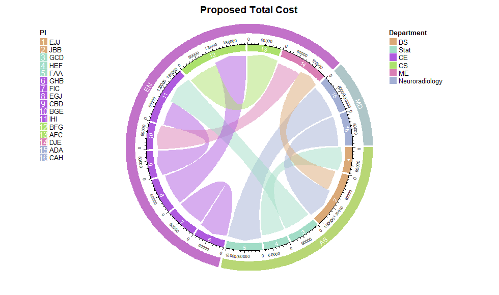
如果你像我一样有点强迫症,你也可以将 sector.numeric.index 添加到扇区中,并在旁边添加一个图例,这样看起来会更好一点,例如 this,只是我的 2 美分!
我需要一些帮助来调整 circlize 包中 chordDiagram() 的高亮扇区。
我正在处理渔业上岸量数据。渔船在一个港口(母港PORT_DE)开始航行,并在另一个港口(着陆港PORT_LA)卸下渔获。我正在处理以吨为单位的扇贝活重(着陆量 SCALLOP_W)。这是数据框的一个简单示例:
PORT_DE PORT_LA SCALLOP_W
1 Aberdeen Aberdeen 116
2 Barrow Barrow 98
3 Douglas Barrow 127
4 Kirkcudbright Barrow 113
5 Brixham Brixham 69
6 Buckie Buckie 180
每个端口 (Name_short) 都按地区 (Region_lb) 和国家 (Country_lb) 标记。示例如下。
Name_short Country_lb Region_lb
1 Scalloway Scotland Shetland Isles
2 Scrabster Scotland North Coast
3 Buckie Scotland Moray Firth
4 Fraserburgh Scotland Moray Firth
5 Aberdeen Scotland North East
使用 circilze 包,我生成了一个自定义的 chordDiagram 来可视化端口之间的着陆流程。我已经调整了大部分设置,包括同一国家的端口分组,通过调整扇区之间的间距(参见 gap.after 设置)。这是我的和弦图的当前形式,
除了最后按国家/地区突出显示部门之外,我几乎已经制作出了我想要的东西。我正在尝试使用 highlight.sector() 来突出显示同一国家/地区的端口,但我无法调整突出显示部分的宽度或位置。目前,国家部门与所有其他标签重叠。下面的示例:
Please note that there are different colours between the two figures as colours are randomly generated.
你能帮我做最后的调整吗?
生成下图的代码:
# calculate gaps by country;
# 1 degree between ports, 10 degree between countries
gaps <- rep(1, nrow(port_coords))
gaps[cumsum(as.numeric(tapply(port_coords$Name_short, port_coords$Country_lb, length)))] <- 10
# edit initialising parameters
circos.par(canvas.ylim=c(-1.5,1.5), # edit canvas size
gap.after = gaps, # adjust gaps between regions
track.margin = c(0.01, 0)) # adjust bottom and top margin
# (blank area out of the plotting regio)
# Plot chord diagram
chordDiagram(m,
# manual order of sectors
order = port_coords$Name_short,
# plot only grid (no labels, no axis)
annotationTrack = "grid",
preAllocateTracks = 1,
# adjust grid width and spacing
annotationTrackHeight = c(0.03, 0.01),
# add directionality
directional=1,
direction.type = c("diffHeight", "arrows"),
link.arr.type = "big.arrow",
# adjust the starting end of the link
diffHeight = -uh(1, "mm"),
# adjust height of all links
h.ratio = 0.8,
# add link border
link.lwd = 1, link.lty = 1, link.border="gray35"
)
# add labels and axis manually
circos.trackPlotRegion(track.index = 1, panel.fun = function(x, y) {
xlim = get.cell.meta.data("xlim")
ylim = get.cell.meta.data("ylim")
sector.name = get.cell.meta.data("sector.index")
# print labels & text size (cex)
circos.text(mean(xlim), ylim[1] + .7, sector.name,
facing = "clockwise", niceFacing = TRUE, adj = c(0, 0.5), cex=0.6)
# print axis
circos.axis(h = "top", labels.cex = 0.5, major.tick.percentage = 0.2,
sector.index = sector.name, track.index = 2)
}, bg.border = NA)
# add additional track to enhance the visual effect of different groups
# Scotland
highlight.sector(port_coords$Name_short[which(port_coords$Country_lb == "Scotland")],
track.index = 1, col = "blue",
text = "Scotland", cex = 0.8, text.col = "white", niceFacing = TRUE)
# England
highlight.sector(port_coords$Name_short[which(port_coords$Country_lb == "England")],
track.index = 1, col = "red",
text = "England", cex = 0.8, text.col = "white", niceFacing = TRUE)
# Wales
highlight.sector(port_coords$Name_short[which(port_coords$Country_lb == "Wales")],
track.index = 1, col = "forestgreen",
text = "Wales", cex = 0.8, text.col = "white", niceFacing = TRUE)
# Isle of Man
highlight.sector(port_coords$Name_short[which(port_coords$Country_lb == "Isle of Man")],
track.index = 1, col = "darkred",
text = "Isle of Man", cex = 0.8, text.col = "white", niceFacing = TRUE)
# Rep. Ireland
highlight.sector(port_coords$Name_short[which(port_coords$Country_lb == "Rep. Ireland")],
track.index = 1, col = "darkorange2",
text = "Ireland", cex = 0.8, text.col = "white", niceFacing = TRUE)
# N.Ireland
highlight.sector(port_coords$Name_short[which(port_coords$Country_lb == "N.Ireland")],
track.index = 1, col = "magenta4",
text = "N. Ireland", cex = 0.8, text.col = "white", niceFacing = TRUE)
# re-set circos parameters
circos.clear()
我已经尝试了一段时间来寻找解决方案。我现在已经设法通过调整默认轨道边距和默认轨道高度来调整 highlight.sector() 的位置和宽度。
我通过在 circos.par() 步骤的初始化中指定 track.margin 和 track.height 参数来完成此操作。
最终产品如下所示。代码在最后答案。
# calculate gaps by country;
# 1 degree between ports, 10 degree between countries
gaps <- rep(1, nrow(port_coords))
gaps[cumsum(as.numeric(tapply(port_coords$Name_short, port_coords$Country_lb, length)))] <- 10
# edit initialising parameters
circos.par(canvas.ylim=c(-1.5,1.5), # edit canvas size
gap.after = gaps, # adjust gaps between regions
track.margin = c(0.01, 0.05), # adjust bottom and top margin
# track.margin = c(0.01, 0.1)
track.height = 0.05)
# Plot chord diagram
chordDiagram(m,
# manual order of sectors
order = port_coords$Name_short,
# plot only grid (no labels, no axis)
annotationTrack = "grid",
# annotationTrack = NULL,
preAllocateTracks = 1,
# adjust grid width and spacing
annotationTrackHeight = c(0.03, 0.01),
# add directionality
directional=1,
direction.type = c("diffHeight", "arrows"),
link.arr.type = "big.arrow",
# adjust the starting end of the link
diffHeight = -uh(1, "mm"),
# adjust height of all links
h.ratio = 0.8,
# add link border
link.lwd = 1, link.lty = 1, link.border="gray35"
# track.margin = c(0.01, 0.1)
)
# Scotland
highlight.sector(port_coords$Name_short[which(port_coords$Country_lb == "Scotland")],
track.index = 1, col = "blue2",
text = "Scotland", cex = 1, text.col = "white",
niceFacing = TRUE, font=2)
# England
highlight.sector(port_coords$Name_short[which(port_coords$Country_lb == "England")],
track.index = 1, col = "red2",
text = "England", cex = 1, text.col = "white",
niceFacing = TRUE, font=2)
# Wales
highlight.sector(port_coords$Name_short[which(port_coords$Country_lb == "Wales")],
track.index = 1, col = "springgreen4",
text = "Wales", cex = 1, text.col = "white",
niceFacing = TRUE, font=2)
# Isle of Man
highlight.sector(port_coords$Name_short[which(port_coords$Country_lb == "Isle of Man")],
track.index = 1, col = "orangered4",
text = "Isle of Man", cex = 1, text.col = "white",
niceFacing = TRUE, font=2)
# Rep. Ireland
highlight.sector(port_coords$Name_short[which(port_coords$Country_lb == "Rep. Ireland")],
track.index = 1, col = "darkorange3",
text = "Ireland", cex = 1, text.col = "white",
niceFacing = TRUE, font=2)
# N.Ireland
highlight.sector(port_coords$Name_short[which(port_coords$Country_lb == "N.Ireland")],
track.index = 1, col = "magenta4",
text = "NI", cex = 1, text.col = "white",
niceFacing = TRUE, font=2)
# add labels and axis manually
circos.trackPlotRegion(track.index = 1, panel.fun = function(x, y) {
xlim = get.cell.meta.data("xlim")
ylim = get.cell.meta.data("ylim")
sector.name = get.cell.meta.data("sector.index")
# print labels & text size (cex)
# circos.text(mean(xlim), ylim[1] + .7, sector.name,
# facing = "clockwise", niceFacing = TRUE, adj = c(0, 0.5), cex=0.6)
circos.text(mean(xlim), ylim[1] + 2, sector.name,
facing = "clockwise", niceFacing = TRUE, adj = c(0, 0.5), cex=0.6)
# print axis
circos.axis(h = "bottom", labels.cex = 0.5,
# major.tick.percentage = 0.05,
major.tick.length = 0.6,
sector.index = sector.name, track.index = 2)
}, bg.border = NA)
# re-set circos parameters
circos.clear()
如果你像我一样有点强迫症,你也可以将 sector.numeric.index 添加到扇区中,并在旁边添加一个图例,这样看起来会更好一点,例如 this,只是我的 2 美分!