Tidymodels - 帮助评估通过配方制作的回归模型
Tidymodels - Help evaluating regression models made via recipes
我正在处理有关工资的当前 tidytuesday 数据,并尝试创建一个包含 tidymodels 和 recipes 的模型。我想使用食谱代码根据许多其他因素预测薪水,但我 运行 遇到了问题。
问题 1 - 我的食谱说有空行,但我不知道如何弄清楚。这不会报错,所以也许这不是问题。
问题 2 - 了解我的模型实际做了什么以及如何可视化性能。我想根据初始数据绘制模型性能。这是我的目标示例:https://indescribled.files.wordpress.com/2021/05/image-17.png?w=782
我不明白如何在我的食谱中使用预测功能。 juice(rec) 少于 1000 行,而测试数据约为 6000。也许我在倒着看,但有人能给我指出正确的方向吗?
下面的代码应该是我的精确复制。
library(tidymodels)
library(tidyverse)

salary_raw <- readr::read_csv('https://raw.githubusercontent.com/rfordatascience/tidytuesday/master/data/2021/2021-05-18/survey.csv')

# Could not figure out tidy way to do this
salary_raw$other_monetary_comp[is.na(salary_raw$other_monetary_comp)] <- 0
salary_raw$other_monetary_comp <- as.numeric(salary_raw$other_monetary_comp)

# Filter and convert to USD
# The mutations to industry were because of other errors, they may not be needed

salary_modeling <- salary_raw %>%
  filter(
    how_old_are_you %in% c("55-64","45-54","35-44","25-34","18-24"),
    currency %in% c("AUD/NZD","CAD","EUR","GBP","USD")
  ) %>%
  mutate(annual_salary = case_when(
    currency == "USD" ~ annual_salary * 1.00,
    currency == "GBP" ~ annual_salary * 1.42,
    currency == "AUD/NZD" ~ annual_salary * 0.75,
    currency == "CAD" ~ annual_salary * 0.83,
    currency == "EUR" ~ annual_salary * 1.22
  )) %>%
  mutate(other_monetary_comp = case_when(
    currency == "USD" ~ other_monetary_comp * 1.00,
    currency == "GBP" ~ other_monetary_comp * 1.42,
    currency == "AUD/NZD" ~ other_monetary_comp * 0.75,
    currency == "CAD" ~ other_monetary_comp * 0.83,
    currency == "EUR" ~ other_monetary_comp * 1.22
  )) %>%
  rename(age = how_old_are_you,
         prof_exp = overall_years_of_professional_experience,
         field_exp = years_of_experience_in_field,
         education = highest_level_of_education_completed
  ) %>%
  mutate(total_comp = annual_salary + other_monetary_comp) %>%
  filter(total_comp > 10000,
         total_comp < 350000)%>%
  mutate(gender = case_when(
    gender == "Prefer not to answer" ~ "Other or prefer not to answer",
    TRUE ~ gender
  )) %>%
  mutate(industry = case_when(
    industry == "Biotech pharmaceuticals" ~ "Biotech",
    industry == "Consumer Packaged Goods" ~ "Consumer packaged goods ",
    industry == "Real Estate Development" ~ "Real Estate",
    TRUE ~ industry
  ))

# Create initial splits

set.seed(123)
salary_split <- initial_split(salary_modeling)
salary_train <- training(salary_split)
salary_test <- testing(salary_split)

# I want to predict total comp with many of the other variables, listed below. Here is my logic
# downsample is because there are a lot more women than men in the data, unsure if necessary
# log is to many data more interpretable, not necessary
# an error message told me to use novel
# unknown is to change NA to unknown as far as I understand
# other is to change values that are less than 5% of the total dataset to "Other"
# unsure what the purpose of dummy is, but it seems to be necessary for modeling

rec <- salary_train %>%
  recipe(total_comp ~ age + gender + field_exp + race + industry + job_title) %>%
  themis::step_downsample(gender) %>%
  step_log(total_comp, base = 2) %>%
  step_novel(race, industry) %>%
  step_unknown(race, industry, gender) %>%
  step_other(race, industry, job_title, threshold = .005) %>%
  step_dummy(all_nominal(), -all_outcomes()) %>%
  prep()

# ISSUE 1 - Running rec says that there are 19,081 data points and 226 incomplete rows. I do not know how to fix the incomplete rows

test_proc <- bake(rec, new_data = salary_test)

# Linear model ------------------------------------------------------------

lm_spec <- linear_reg() %>%
  set_engine("lm")

lm_fitted <- lm_spec %>%
  fit(total_comp ~ ., data = juice(rec))
tidy(lm_fitted)

# RF MODEL ----------------------------------------------------------------

rf_spec <- rand_forest(mode = "regression", trees = 1500) %>%
  set_engine("ranger")

rf_fit <- rf_spec %>%
  fit(total_comp ~ .,
      data = juice(rec))
rf_fit

# QUESTIONS BEGIN HERE --------------------------------------------------------------------------------------------------------------------------------------------------

# Need to figure out what new data is for this portion
# I think it is juice(rec), but it seems weird to me
# juice(rec) is only about 900 rows while test_proc is multiple thousand. testing data should be smaller than training
asdf <- juice(rec)

results_train <- lm_fitted %>%
  predict(new_data = asdf) %>%
  mutate(
    truth = asdf$total_comp,
    model = "lm"
  ) %>%
  bind_rows(rf_fit %>%
              predict(new_data = asdf) %>%
              mutate(
                truth = asdf$total_comp,
                model = "rf"
              ))
results_train

# Is the newdata and test proc correct?
results_test <- lm_fitted %>%
  predict(new_data = test_proc) %>%
  mutate(
    truth = test_proc$total_comp,
    model = "lm"
  ) %>%
  bind_rows(rf_fit %>%
              predict(new_data = test_proc) %>%
              mutate(
                truth = test_proc$total_comp,
                model = "rf"
              ))
results_test

# Goal is to run the following code to visualize the predictions, the code below probably will do nothing right now unless the two dataframes above are correct

results_test %>%
  mutate(train = "testing") %>%
  bind_rows(results_train %>%
              mutate(train = "training")) %>%
  ggplot(aes(truth, .pred, color = model)) +
    geom_abline(lty = 2, color = "gray80", size = 1.5) +
    geom_point(alpha = .75) +
    facet_wrap(~train)
看来你进展顺利!
library(tidymodels)
library(tidyverse)

salary_raw <- readr::read_csv('https://raw.githubusercontent.com/rfordatascience/tidytuesday/master/data/2021/2021-05-18/survey.csv')
#>
#> ── Column specification ────────────────────────────────────────────────────────
#> cols(
#>   timestamp = col_character(),
#>   how_old_are_you = col_character(),
#>   industry = col_character(),
#>   job_title = col_character(),
#>   additional_context_on_job_title = col_character(),
#>   annual_salary = col_double(),
#>   other_monetary_comp = col_character(),
#>   currency = col_character(),
#>   currency_other = col_character(),
#>   additional_context_on_income = col_character(),
#>   country = col_character(),
#>   state = col_character(),
#>   city = col_character(),
#>   overall_years_of_professional_experience = col_character(),
#>   years_of_experience_in_field = col_character(),
#>   highest_level_of_education_completed = col_character(),
#>   gender = col_character(),
#>   race = col_character()
#> )

salary_modeling <- salary_raw %>%
  replace_na(list(other_monetary_comp = 0)) %>%
  filter(
    how_old_are_you %in% c("55-64","45-54","35-44","25-34","18-24"),
    currency %in% c("AUD/NZD","CAD","EUR","GBP","USD")
  ) %>%
  mutate(annual_salary = case_when(
    currency == "USD" ~ annual_salary * 1.00,
    currency == "GBP" ~ annual_salary * 1.42,
    currency == "AUD/NZD" ~ annual_salary * 0.75,
    currency == "CAD" ~ annual_salary * 0.83,
    currency == "EUR" ~ annual_salary * 1.22
  )) %>%
  mutate(other_monetary_comp = parse_number(other_monetary_comp),
         other_monetary_comp = case_when(
    currency == "USD" ~ other_monetary_comp * 1.00,
    currency == "GBP" ~ other_monetary_comp * 1.42,
    currency == "AUD/NZD" ~ other_monetary_comp * 0.75,
    currency == "CAD" ~ other_monetary_comp * 0.83,
    currency == "EUR" ~ other_monetary_comp * 1.22
  )) %>%
  rename(age = how_old_are_you,
         prof_exp = overall_years_of_professional_experience,
         field_exp = years_of_experience_in_field,
         education = highest_level_of_education_completed
  ) %>%
  mutate(total_comp = annual_salary + other_monetary_comp) %>%
  filter(total_comp > 10000,
         total_comp < 350000) %>%
  mutate(gender = case_when(
    gender == "Prefer not to answer" ~ "Other or prefer not to answer",
    TRUE ~ gender
  )) %>%
  mutate(industry = case_when(
    industry == "Biotech pharmaceuticals" ~ "Biotech",
    industry == "Consumer Packaged Goods" ~ "Consumer packaged goods ",
    industry == "Real Estate Development" ~ "Real Estate",
    TRUE ~ industry
  ))

set.seed(123)
salary_split <- initial_split(salary_modeling)
salary_train <- training(salary_split)
salary_test <- testing(salary_split)

rec <- salary_train %>%
  recipe(total_comp ~ age + gender + field_exp + race + industry + job_title) %>%
  themis::step_downsample(gender) %>%
  step_log(total_comp, base = 2) %>%
  step_novel(race, industry) %>%
  step_unknown(race, industry, gender) %>%
  step_other(race, industry, job_title, threshold = 0.005) %>%
  step_dummy(all_nominal_predictors())
这里的配方说训练数据有不完整的行,因为有缺失数据;这就是你使用 step_unknown() 的原因,我猜。
prep(rec)
#> Data Recipe
#>
#> Inputs:
#>
#>       role #variables
#>    outcome          1
#>  predictor          6
#>
#> Training data contained 19080 data points and 235 incomplete rows.
#>
#> Operations:
#>
#> Down-sampling based on gender [trained]
#> Log transformation on total_comp [trained]
#> Novel factor level assignment for race, industry [trained]
#> Unknown factor level assignment for race, industry, gender [trained]
#> Collapsing factor levels for race, industry, job_title [trained]
#> Dummy variables from age, gender, field_exp, race, industry, job_title [trained]
这里经过处理的训练集因为降采样,不再有那么多观察值;我们不对测试集应用下采样,因为我们想计算测试集上的指标,因为它们会出现在“野外”。
train_proc <- rec %>% prep() %>% bake(new_data = NULL)
test_proc  <- rec %>% prep() %>% bake(new_data = salary_test)
dim(train_proc)
#> [1] 878  57
dim(test_proc)
#> [1] 6361   57


lm_fitted <- linear_reg() %>%
  set_engine("lm") %>%
  fit(total_comp ~ ., data = train_proc)

rf_fitted <- rand_forest(mode = "regression", trees = 1500) %>%
  set_engine("ranger") %>%
  fit(total_comp ~ ., data = train_proc)
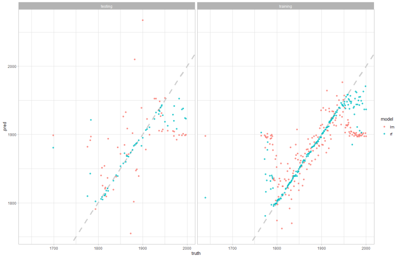
我会尝试使用 augment() 函数来制作您的可视化
bind_rows(
  augment(lm_fitted, new_data = train_proc) %>% mutate(model = "lm", train = "train"),
  augment(rf_fitted, new_data = train_proc) %>% mutate(model = "rf", train = "train"),
  augment(lm_fitted, new_data = test_proc) %>% mutate(model = "lm", train = "test"),
  augment(rf_fitted, new_data = test_proc) %>% mutate(model = "rf", train = "test")
) %>%
  ggplot(aes(total_comp, .pred, color = model)) +
  geom_abline(lty = 2, color = "gray80", size = 1.5) +
  geom_point(alpha = .5) +
  facet_wrap(~ train)
由 reprex package (v2.0.0)
于 2021-05-24 创建
我正在处理有关工资的当前 tidytuesday 数据,并尝试创建一个包含 tidymodels 和 recipes 的模型。我想使用食谱代码根据许多其他因素预测薪水,但我 运行 遇到了问题。
问题 1 - 我的食谱说有空行,但我不知道如何弄清楚。这不会报错,所以也许这不是问题。
问题 2 - 了解我的模型实际做了什么以及如何可视化性能。我想根据初始数据绘制模型性能。这是我的目标示例:https://indescribled.files.wordpress.com/2021/05/image-17.png?w=782
我不明白如何在我的食谱中使用预测功能。 juice(rec) 少于 1000 行,而测试数据约为 6000。也许我在倒着看,但有人能给我指出正确的方向吗?
下面的代码应该是我的精确复制。
library(tidymodels)
library(tidyverse)
salary_raw <- readr::read_csv('https://raw.githubusercontent.com/rfordatascience/tidytuesday/master/data/2021/2021-05-18/survey.csv')
# Could not figure out tidy way to do this
salary_raw$other_monetary_comp[is.na(salary_raw$other_monetary_comp)] <- 0
salary_raw$other_monetary_comp <- as.numeric(salary_raw$other_monetary_comp)
# Filter and convert to USD
# The mutations to industry were because of other errors, they may not be needed
salary_modeling <- salary_raw %>%
filter(
how_old_are_you %in% c("55-64","45-54","35-44","25-34","18-24"),
currency %in% c("AUD/NZD","CAD","EUR","GBP","USD")
) %>%
mutate(annual_salary = case_when(
currency == "USD" ~ annual_salary * 1.00,
currency == "GBP" ~ annual_salary * 1.42,
currency == "AUD/NZD" ~ annual_salary * 0.75,
currency == "CAD" ~ annual_salary * 0.83,
currency == "EUR" ~ annual_salary * 1.22
)) %>%
mutate(other_monetary_comp = case_when(
currency == "USD" ~ other_monetary_comp * 1.00,
currency == "GBP" ~ other_monetary_comp * 1.42,
currency == "AUD/NZD" ~ other_monetary_comp * 0.75,
currency == "CAD" ~ other_monetary_comp * 0.83,
currency == "EUR" ~ other_monetary_comp * 1.22
)) %>%
rename(age = how_old_are_you,
prof_exp = overall_years_of_professional_experience,
field_exp = years_of_experience_in_field,
education = highest_level_of_education_completed
) %>%
mutate(total_comp = annual_salary + other_monetary_comp) %>%
filter(total_comp > 10000,
total_comp < 350000)%>%
mutate(gender = case_when(
gender == "Prefer not to answer" ~ "Other or prefer not to answer",
TRUE ~ gender
)) %>%
mutate(industry = case_when(
industry == "Biotech pharmaceuticals" ~ "Biotech",
industry == "Consumer Packaged Goods" ~ "Consumer packaged goods ",
industry == "Real Estate Development" ~ "Real Estate",
TRUE ~ industry
))
# Create initial splits
set.seed(123)
salary_split <- initial_split(salary_modeling)
salary_train <- training(salary_split)
salary_test <- testing(salary_split)
# I want to predict total comp with many of the other variables, listed below. Here is my logic
# downsample is because there are a lot more women than men in the data, unsure if necessary
# log is to many data more interpretable, not necessary
# an error message told me to use novel
# unknown is to change NA to unknown as far as I understand
# other is to change values that are less than 5% of the total dataset to "Other"
# unsure what the purpose of dummy is, but it seems to be necessary for modeling
rec <- salary_train %>%
recipe(total_comp ~ age + gender + field_exp + race + industry + job_title) %>%
themis::step_downsample(gender) %>%
step_log(total_comp, base = 2) %>%
step_novel(race, industry) %>%
step_unknown(race, industry, gender) %>%
step_other(race, industry, job_title, threshold = .005) %>%
step_dummy(all_nominal(), -all_outcomes()) %>%
prep()
# ISSUE 1 - Running rec says that there are 19,081 data points and 226 incomplete rows. I do not know how to fix the incomplete rows
test_proc <- bake(rec, new_data = salary_test)
# Linear model ------------------------------------------------------------
lm_spec <- linear_reg() %>%
set_engine("lm")
lm_fitted <- lm_spec %>%
fit(total_comp ~ ., data = juice(rec))
tidy(lm_fitted)
# RF MODEL ----------------------------------------------------------------
rf_spec <- rand_forest(mode = "regression", trees = 1500) %>%
set_engine("ranger")
rf_fit <- rf_spec %>%
fit(total_comp ~ .,
data = juice(rec))
rf_fit
# QUESTIONS BEGIN HERE --------------------------------------------------------------------------------------------------------------------------------------------------
# Need to figure out what new data is for this portion
# I think it is juice(rec), but it seems weird to me
# juice(rec) is only about 900 rows while test_proc is multiple thousand. testing data should be smaller than training
asdf <- juice(rec)
results_train <- lm_fitted %>%
predict(new_data = asdf) %>%
mutate(
truth = asdf$total_comp,
model = "lm"
) %>%
bind_rows(rf_fit %>%
predict(new_data = asdf) %>%
mutate(
truth = asdf$total_comp,
model = "rf"
))
results_train
# Is the newdata and test proc correct?
results_test <- lm_fitted %>%
predict(new_data = test_proc) %>%
mutate(
truth = test_proc$total_comp,
model = "lm"
) %>%
bind_rows(rf_fit %>%
predict(new_data = test_proc) %>%
mutate(
truth = test_proc$total_comp,
model = "rf"
))
results_test
# Goal is to run the following code to visualize the predictions, the code below probably will do nothing right now unless the two dataframes above are correct
results_test %>%
mutate(train = "testing") %>%
bind_rows(results_train %>%
mutate(train = "training")) %>%
ggplot(aes(truth, .pred, color = model)) +
geom_abline(lty = 2, color = "gray80", size = 1.5) +
geom_point(alpha = .75) +
facet_wrap(~train)
看来你进展顺利!
library(tidymodels)
library(tidyverse)
salary_raw <- readr::read_csv('https://raw.githubusercontent.com/rfordatascience/tidytuesday/master/data/2021/2021-05-18/survey.csv')
#>
#> ── Column specification ────────────────────────────────────────────────────────
#> cols(
#> timestamp = col_character(),
#> how_old_are_you = col_character(),
#> industry = col_character(),
#> job_title = col_character(),
#> additional_context_on_job_title = col_character(),
#> annual_salary = col_double(),
#> other_monetary_comp = col_character(),
#> currency = col_character(),
#> currency_other = col_character(),
#> additional_context_on_income = col_character(),
#> country = col_character(),
#> state = col_character(),
#> city = col_character(),
#> overall_years_of_professional_experience = col_character(),
#> years_of_experience_in_field = col_character(),
#> highest_level_of_education_completed = col_character(),
#> gender = col_character(),
#> race = col_character()
#> )
salary_modeling <- salary_raw %>%
replace_na(list(other_monetary_comp = 0)) %>%
filter(
how_old_are_you %in% c("55-64","45-54","35-44","25-34","18-24"),
currency %in% c("AUD/NZD","CAD","EUR","GBP","USD")
) %>%
mutate(annual_salary = case_when(
currency == "USD" ~ annual_salary * 1.00,
currency == "GBP" ~ annual_salary * 1.42,
currency == "AUD/NZD" ~ annual_salary * 0.75,
currency == "CAD" ~ annual_salary * 0.83,
currency == "EUR" ~ annual_salary * 1.22
)) %>%
mutate(other_monetary_comp = parse_number(other_monetary_comp),
other_monetary_comp = case_when(
currency == "USD" ~ other_monetary_comp * 1.00,
currency == "GBP" ~ other_monetary_comp * 1.42,
currency == "AUD/NZD" ~ other_monetary_comp * 0.75,
currency == "CAD" ~ other_monetary_comp * 0.83,
currency == "EUR" ~ other_monetary_comp * 1.22
)) %>%
rename(age = how_old_are_you,
prof_exp = overall_years_of_professional_experience,
field_exp = years_of_experience_in_field,
education = highest_level_of_education_completed
) %>%
mutate(total_comp = annual_salary + other_monetary_comp) %>%
filter(total_comp > 10000,
total_comp < 350000) %>%
mutate(gender = case_when(
gender == "Prefer not to answer" ~ "Other or prefer not to answer",
TRUE ~ gender
)) %>%
mutate(industry = case_when(
industry == "Biotech pharmaceuticals" ~ "Biotech",
industry == "Consumer Packaged Goods" ~ "Consumer packaged goods ",
industry == "Real Estate Development" ~ "Real Estate",
TRUE ~ industry
))
set.seed(123)
salary_split <- initial_split(salary_modeling)
salary_train <- training(salary_split)
salary_test <- testing(salary_split)
rec <- salary_train %>%
recipe(total_comp ~ age + gender + field_exp + race + industry + job_title) %>%
themis::step_downsample(gender) %>%
step_log(total_comp, base = 2) %>%
step_novel(race, industry) %>%
step_unknown(race, industry, gender) %>%
step_other(race, industry, job_title, threshold = 0.005) %>%
step_dummy(all_nominal_predictors())
这里的配方说训练数据有不完整的行,因为有缺失数据;这就是你使用 step_unknown() 的原因,我猜。
prep(rec)
#> Data Recipe
#>
#> Inputs:
#>
#> role #variables
#> outcome 1
#> predictor 6
#>
#> Training data contained 19080 data points and 235 incomplete rows.
#>
#> Operations:
#>
#> Down-sampling based on gender [trained]
#> Log transformation on total_comp [trained]
#> Novel factor level assignment for race, industry [trained]
#> Unknown factor level assignment for race, industry, gender [trained]
#> Collapsing factor levels for race, industry, job_title [trained]
#> Dummy variables from age, gender, field_exp, race, industry, job_title [trained]
这里经过处理的训练集因为降采样,不再有那么多观察值;我们不对测试集应用下采样,因为我们想计算测试集上的指标,因为它们会出现在“野外”。
train_proc <- rec %>% prep() %>% bake(new_data = NULL)
test_proc <- rec %>% prep() %>% bake(new_data = salary_test)
dim(train_proc)
#> [1] 878 57
dim(test_proc)
#> [1] 6361 57
lm_fitted <- linear_reg() %>%
set_engine("lm") %>%
fit(total_comp ~ ., data = train_proc)
rf_fitted <- rand_forest(mode = "regression", trees = 1500) %>%
set_engine("ranger") %>%
fit(total_comp ~ ., data = train_proc)
我会尝试使用 augment() 函数来制作您的可视化
bind_rows(
augment(lm_fitted, new_data = train_proc) %>% mutate(model = "lm", train = "train"),
augment(rf_fitted, new_data = train_proc) %>% mutate(model = "rf", train = "train"),
augment(lm_fitted, new_data = test_proc) %>% mutate(model = "lm", train = "test"),
augment(rf_fitted, new_data = test_proc) %>% mutate(model = "rf", train = "test")
) %>%
ggplot(aes(total_comp, .pred, color = model)) +
geom_abline(lty = 2, color = "gray80", size = 1.5) +
geom_point(alpha = .5) +
facet_wrap(~ train)
由 reprex package (v2.0.0)
于 2021-05-24 创建