如何在回归模型的ggplot中为另一个因素添加形状
How to add shapes for another factor in ggplot for regression model
我正在尝试为回归模型添加形状。这是示例:
library(ggpubr)
data(iris)
iris$ran <- as.factor(rep(c(1:2), each = 75))
fit <- lm(Sepal.Length ~ Petal.Width+Species+ran, data = iris)
ggplot(fit$model, aes_string(x = names(fit$model)[2], y = names(fit$model)[1],
color=names(fit$model)[3], shape=names(fit$model)[4])) +
geom_point() +
geom_smooth(aes_string(fill = names(fit$model)[3], color = names(fit$model)[3]),
method = "lm", col= "red", fullrange = TRUE) +
labs(x=expression(paste("Petal Width")),
     y=expression(paste("Sepal Length")),
     caption = paste("R2 =",signif(summary(fit)$r.squared, 2),
                     "\tAdj R2 =",signif(summary(fit)$adj.r.squared, 2),
                     "\tIntercept =",signif(fit$coef[[1]],2 ),
                     "\tSlope =",signif(fit$coef[[2]], 2),
                     "\tP =",signif(summary(fit)$coef[2,4], 2)))+
theme_classic2(base_size = 14)
我得到一个图,其中每个因素都有 4 条直线。我宁愿只为“物种”设置线性回归线,但为“运行”设置不同的形状(不向图中添加“运行”的回归线)。
此外,我还打算将“R2”更改为 R^2,我无法使用当前脚本将其更改为“Random”-“Factor1”和“Factor2”的 运行 图例".
预先感谢您的帮助。
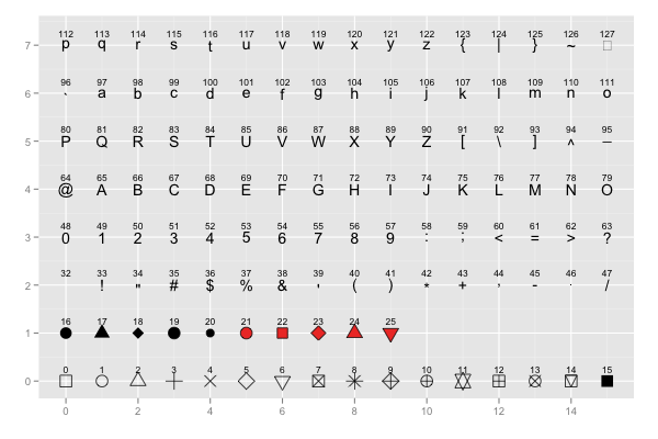
你可以scale_shape_manual根据这个chart修改形状符号。
此外,您可以直接使用 unicode 字符 ² 通过从 here:
复制它来打印系数
library(ggpubr)
#> Loading required package: ggplot2
library(tidyverse)
library(latex2exp)

iris$ran <- as.factor(rep(c(1:2), each = 75))
fit <- lm(Sepal.Length ~ Petal.Width + Species + ran, data = iris)

fit$model %>%
  ggplot(aes_string(
    x = names(fit$model)[2], y = names(fit$model)[1]
  )) +
  geom_point(aes_string(shape = names(fit$model)[4]), size = 2.5) +
  geom_smooth(aes_string(color = names(fit$model)[3]),
    method = "lm", fullrange = TRUE, se = FALSE
  ) +
  theme_classic2(base_size = 14) +
  scale_shape_manual(values = c(17, 18)) +
  labs(
    x = "Petal Width",
    y = "Sepal Length",
    caption = paste(
      "R² =", signif(summary(fit)$r.squared, 2),
      "\tAdj R²=", signif(summary(fit)$adj.r.squared, 2),
      "\tIntercept =", signif(fit$coef[[1]], 2),
      "\tSlope =", signif(fit$coef[[2]], 2),
      "\tP =", signif(summary(fit)$coef[2, 4], 2)
    )
  )
#> `geom_smooth()` using formula 'y ~ x'
由 reprex package (v2.0.1)
于 2021-09-09 创建
为了阐明回归线,我在 geom_smooth 中设置了 se = FALSE。
我认为这个备选答案更简单。可以使用 fullrange = TRUE 和 se = FALSE 而不是使用这种方法对点进行着色,但这会产生严重歪曲数据的图。即使这不会产生相同的标题,我的答案中的代码也会自动显示三个拟合中的每一个的结果,并且它会在不同数量的因子水平下保持不变。
这里以iris数据为例,所以宽和长都是随机变量,可以忽略不计,使用OLS。否则主轴回归会更好,下面的代码可以使用 stat_ma_line() 和 stat_ma_eq() 重写,并稍微调整传递给它们的参数。
library(ggpmisc)
#> Loading required package: ggpp
#> Loading required package: ggplot2
#>
#> Attaching package: 'ggpp'
#> The following object is masked from 'package:ggplot2':
#>
#>     annotate
iris$ran <- factor(rep(c(1:2), each = 75), labels = paste("Factor", 1:2))

ggplot(iris, aes(Petal.Width, Sepal.Length, colour = Species)) +
  geom_point(aes(shape = ran)) +
  stat_poly_line() + # se = FALSE can be added
  stat_poly_eq(aes(label = paste(after_stat(rr.label),
#                                 after_stat(adj.rr.label),
                                 after_stat(eq.label),
                                 after_stat(p.value.label),
#                                 after_stat(n.label),
                                 sep = "*\", \"*"))) +
  labs(x = "Petal Width", y = "Sepal length", shape = "Random") +
  theme_classic(base_size = 14)
由 reprex package (v2.0.1)
于 2021-09-10 创建
我正在尝试为回归模型添加形状。这是示例:
library(ggpubr)
data(iris)
iris$ran <- as.factor(rep(c(1:2), each = 75))
fit <- lm(Sepal.Length ~ Petal.Width+Species+ran, data = iris)
ggplot(fit$model, aes_string(x = names(fit$model)[2], y = names(fit$model)[1],
color=names(fit$model)[3], shape=names(fit$model)[4])) +
geom_point() +
geom_smooth(aes_string(fill = names(fit$model)[3], color = names(fit$model)[3]),
method = "lm", col= "red", fullrange = TRUE) +
labs(x=expression(paste("Petal Width")),
y=expression(paste("Sepal Length")),
caption = paste("R2 =",signif(summary(fit)$r.squared, 2),
"\tAdj R2 =",signif(summary(fit)$adj.r.squared, 2),
"\tIntercept =",signif(fit$coef[[1]],2 ),
"\tSlope =",signif(fit$coef[[2]], 2),
"\tP =",signif(summary(fit)$coef[2,4], 2)))+
theme_classic2(base_size = 14)
我得到一个图,其中每个因素都有 4 条直线。我宁愿只为“物种”设置线性回归线,但为“运行”设置不同的形状(不向图中添加“运行”的回归线)。
此外,我还打算将“R2”更改为 R^2,我无法使用当前脚本将其更改为“Random”-“Factor1”和“Factor2”的 运行 图例".
预先感谢您的帮助。
你可以scale_shape_manual根据这个chart修改形状符号。
此外,您可以直接使用 unicode 字符 ² 通过从 here:
library(ggpubr)
#> Loading required package: ggplot2
library(tidyverse)
library(latex2exp)
iris$ran <- as.factor(rep(c(1:2), each = 75))
fit <- lm(Sepal.Length ~ Petal.Width + Species + ran, data = iris)
fit$model %>%
ggplot(aes_string(
x = names(fit$model)[2], y = names(fit$model)[1]
)) +
geom_point(aes_string(shape = names(fit$model)[4]), size = 2.5) +
geom_smooth(aes_string(color = names(fit$model)[3]),
method = "lm", fullrange = TRUE, se = FALSE
) +
theme_classic2(base_size = 14) +
scale_shape_manual(values = c(17, 18)) +
labs(
x = "Petal Width",
y = "Sepal Length",
caption = paste(
"R² =", signif(summary(fit)$r.squared, 2),
"\tAdj R²=", signif(summary(fit)$adj.r.squared, 2),
"\tIntercept =", signif(fit$coef[[1]], 2),
"\tSlope =", signif(fit$coef[[2]], 2),
"\tP =", signif(summary(fit)$coef[2, 4], 2)
)
)
#> `geom_smooth()` using formula 'y ~ x'
由 reprex package (v2.0.1)
于 2021-09-09 创建为了阐明回归线,我在 geom_smooth 中设置了 se = FALSE。
我认为这个备选答案更简单。可以使用 fullrange = TRUE 和 se = FALSE 而不是使用这种方法对点进行着色,但这会产生严重歪曲数据的图。即使这不会产生相同的标题,我的答案中的代码也会自动显示三个拟合中的每一个的结果,并且它会在不同数量的因子水平下保持不变。
这里以iris数据为例,所以宽和长都是随机变量,可以忽略不计,使用OLS。否则主轴回归会更好,下面的代码可以使用 stat_ma_line() 和 stat_ma_eq() 重写,并稍微调整传递给它们的参数。
library(ggpmisc)
#> Loading required package: ggpp
#> Loading required package: ggplot2
#>
#> Attaching package: 'ggpp'
#> The following object is masked from 'package:ggplot2':
#>
#> annotate
iris$ran <- factor(rep(c(1:2), each = 75), labels = paste("Factor", 1:2))
ggplot(iris, aes(Petal.Width, Sepal.Length, colour = Species)) +
geom_point(aes(shape = ran)) +
stat_poly_line() + # se = FALSE can be added
stat_poly_eq(aes(label = paste(after_stat(rr.label),
# after_stat(adj.rr.label),
after_stat(eq.label),
after_stat(p.value.label),
# after_stat(n.label),
sep = "*\", \"*"))) +
labs(x = "Petal Width", y = "Sepal length", shape = "Random") +
theme_classic(base_size = 14)
由 reprex package (v2.0.1)
于 2021-09-10 创建